
DeepFormFinding
In September 2018, I've had the opportunity to take part of the Advance in Architectural Geometry 2018 at Chalmers University in Göteborg, Sweden. This is the work and experimentations from the workshop "Deep Form Finding".
Similarly to a previous post "HouseOfGan", this workshop explored the implementation of Artificial Intelligences in the architectural world.
This masterclass was given by Jaime de Miguel (PhD candidate in Computer Science & AI at the University of Seville) and Maria Eugenia Villafañe (architect working in the field of structural engineering at Atelier One in London, UK).
Neural networks have now been around for decades. But since very recently, researches have been made in the field of architecture. Let's try to explain very shortly and very naïvely their variants how they works and how we used them throughout the workshop.
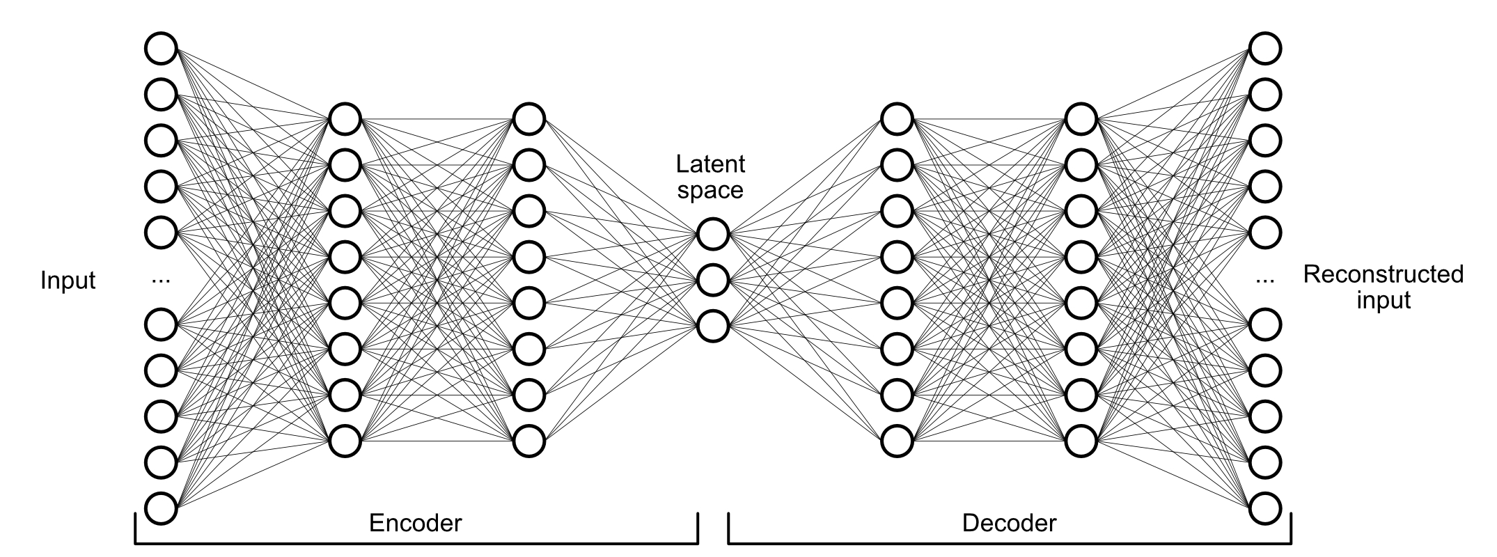
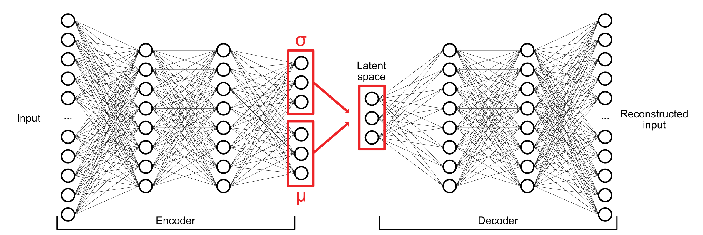
We will explore three types of Neural Networks : Deep Neural networks, Auto-encoder and Variational auto-encoder.
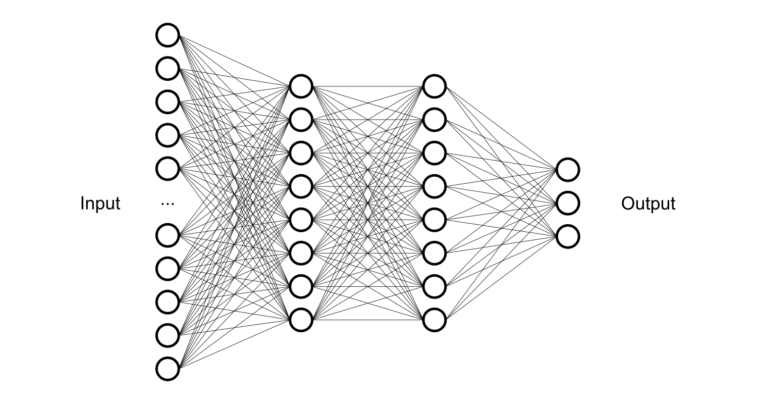


The first one represents the well known neural network graph. This is what we could find behind most of the trained regular machine learning models, with some variations. Besides their aptitude to solve many tasks, as long as they are well trained for the question they are being asked for, this kind of network needs the assistance of a human being to teach them if the produced output is correct or not. But what if a network could train itself?
The Auto-encoder graph works the same way as the Deep neural network, for its left part. However, the right part will (most likely) always be the mirrored structure. This configuration allows the network to (or at least to try to) reconstruct the given input after the data got condensed in the latent space layer. The network uses a Loss function to measure the difference between the reconstructed input from the original input. With this information, it will be able to tweak all the weights and biases that come with the neurons so it can identify which one performs better to recognize certain features from the input. There are multiple Loss functions available and their uses will depend on the given problem.
The last graph, called Variational Auto-encoder, is almost the same as the previous one, but it involves two additional functions in its middle part : a mean function & a standard deviation function (also called Gaussian distribution). This last add on will be the key for the network to be able to generate interpolation between the inputs. This is the type of network that we've been using for the workshop.
Exercice time !
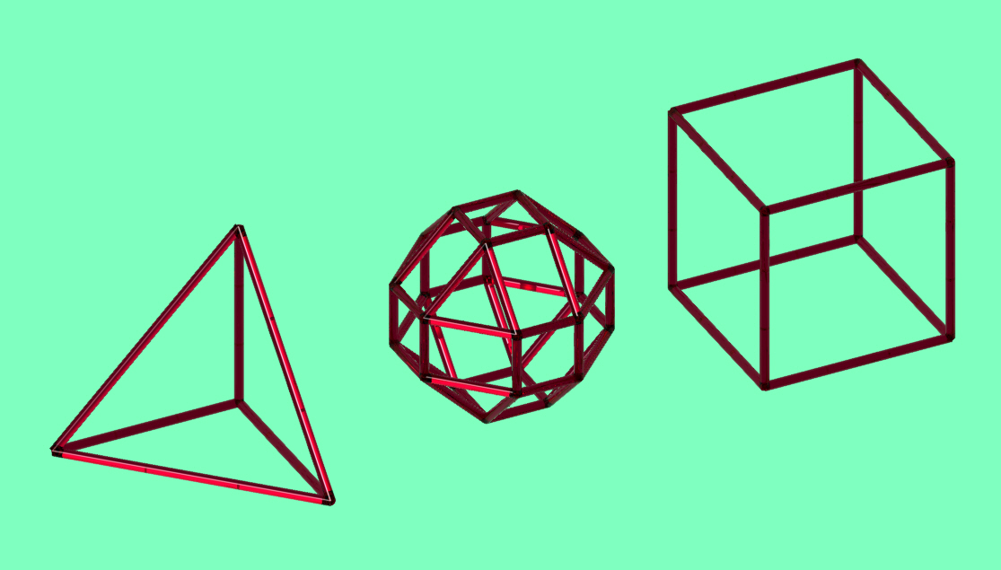
Let's start with a very basic example : a tetrahedron, a sphere-like shape and a squared box. These geometries have been created directly into Rhino.
Unfortunately, neural networks cannot read 3D geometries, but thanks to the great work of Jaime and Maria, we received a Python script that runs through each point of each geometry and creates a list of all the connection vectors. More than that, the script also creates a certain amount of duplicated samples and move them around in a certain desired "fish tank" space. This is necessary for the model to better train itself at targeting the specific features of each of the three geometries (in this case).

Now that the 3D data has been converted into a (super huge) set of vectors (each points, each geometry, each 3000 variations), it's time for us to feed the Variational auto-encoder monster.
For that, Jaime and Maria came up with custom made Keras scripts. Keras is a high-level neural networks API, written in Python and capable of running on top of TensorFlow. Through these scripts we could tweak our variational auto-encoder network's architecture and its settings to explore the way it works and create different sets of output.
This part is were computational power was needed the most. The convergence process, which names the learning process of the network, took around 20 minutes on a mid 2014 macbook pro.
The network's architecture was 6552 : 300 : 300 : 200 : 2 : 2 : 2 : 200 : 300 : 300 : 6552 and ran 25 epochs of 3000 samples of each of the three geometries to give us the following data.


It's now time to re-open Rhino and see what's behind all this data. Here again, Jaime and Maria had prepared a custom script to read the data and translate it into wireframes shapes into Rhino, the same type of wireframe shapes that we first created. In this last step, there were also some settings to choose from. The main one being the threshold point when a vector's value is to be considered as a connection or not.
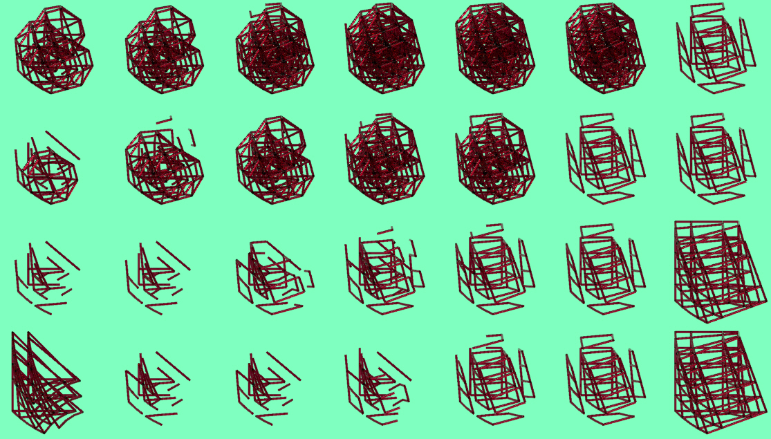
These quite rough geometries are one of the results from the self trained network. It has learned the features from the three geometries I fed him with, and it has been able to interpolate them into a shape gradient-like grid. Other geometries have been tested, with different settings, as you can see below.

Crossover between the CCTV tower and the Battersa building in London - Jaime & Maria
Conclusion
This is an experimental work from a two days workshop, led by two true pioneers of artificial intelligence in the architecture world. Results may be sloppy to be applied yet in an actual creative workflow. Although things go fast… A year ago, none of this (nor the "HouseOfGan" post) had ever been mentioned in the field of architecture. Let's see what future works in this area will bring us !
Special thanks to Jaime, Maria, Chalmers University and all the participants of AAG2018. It has been quite an experience full of interdisciplinary works, researches and new ways of thinking about geometries and architecture itself. Anyone reading this should attend AAG2020 in Paris !
A link to our workshop's results should be available soon on www.sofiaproject.net
Antoine -
